Along with my earlier post on the reshape2 package, I will continue to post my course notes from Data Wrangling and Visualization in R, a graduate-level course I co-taught last semester at Simon Fraser University.
plyr is an R package that makes it simple to split data apart, do
stuff to it, and mash it back together. This is a common
data-manipulation step. Importantly, plyr makes it easy to control the
input and output data format with a consistent syntax.
Or, from the documentation:
“plyr is a set of tools that solves a common set of problems: you need
to break a big problem down into manageable pieces, operate on each
piece and then put all the pieces back together. It’s already possible
to do this with split and the apply functions, but plyr just makes it
all a bit easier…”
This is a very quick introduction to plyr. For more details see Hadley
Wickham’s introductory guide The split-apply-combine strategy for data
analysis. There’s quite a bit of discussion
online in general, and especially on
stackoverflow.com.
Why use apply functions instead of for loops?
The code is cleaner (once you’re familiar with the concept). The code can be easier to code and read, and less error prone because you don’t have to deal with subsetting and you don’t have to deal with saving your results.
applyfunctions can be faster thanforloops, sometimes dramatically.
plyr basics
plyr builds on the built-in apply functions by giving you control
over the input and output formats and keeping the syntax consistent
across all variations. It also adds some niceties like error processing,
parallel processing, and progress bars.
The basic format is two letters followed by ply(). The first letter
refers to the format in and the second to the format out.
The three main letters are:
d= data framea= array (includes matrices)l= list
So, ddply means: take a data frame, split it up, do something to it,
and return a data frame. I find I use this the majority of the time
since I often work with data frames. ldply means: take a list, split
it up, do something to it, and return a data frame. This extends to all
combinations. In the following table, the columns are the input formats
and the rows are the output format:
| object type | data frame | list | array |
|---|---|---|---|
| data frame | ddply |
ldply |
adply |
| list | dlply |
llply |
alply |
| array | daply |
laply |
aaply |
I’ve ignored some less common format options:
m= multi-argument function inputr= replicate a functionntimes._= throw away the output
For plotting, you might find the underscore (_) option useful. It will
do something with the data (say add line segments to a plot) and then
throw away the output (e.g., d_ply()).
Base R apply functions and plyr
plyr provides a consistent and easy-to-work-with format for apply
functions with control over the input and output formats. Some of the
functionality can be duplicated with base R functions (but with less
consistent syntax). Also, few R apply functions work directly with
data frames as input and output and data frames are a common object
class to work with.
Base R apply functions (from a presentation given by Hadley Wickham):
| object type | array | data frame | list | nothing |
|---|---|---|---|---|
| array | apply |
. | . | . |
| data frame | . | aggregate |
by |
. |
| list | sapply |
. | lapply |
. |
| n replicates | replicate |
. | replicate |
. |
| function arguments | mapply |
. | mapply |
. |
A general example with plyr
Let’s take a simple example. We’ll take a data frame, split it up by
year, calculate the coefficient of variation of the count, and
return a data frame. This could easily be done on one line, but I’m
expanding it here to show the format a more complex function could take.
set.seed(1)
d <- data.frame(year = rep(2000:2002, each = 3),
  count = round(runif(9, 0, 20)))
print(d)
## year count
## 1 2000 5
## 2 2000 7
## 3 2000 11
## 4 2001 18
## 5 2001 4
## 6 2001 18
## 7 2002 19
## 8 2002 13
## 9 2002 13library(plyr)
ddply(d, "year", function(x) {
mean.count <- mean(x$count)
sd.count <- sd(x$count)
cv <- sd.count/mean.count
data.frame(cv.count = cv)
})## year cv.count
## 1 2000 0.3984848
## 2 2001 0.6062178
## 3 2002 0.2309401transform and summarise
It is often convenient to use these functions within one of the **ply
functions. transform acts as it would normally as the base R function and
modifies an existing data frame. summarise creates a new condensed data
frame.
ddply(d, "year", summarise, mean.count = mean(count))## year mean.count
## 1 2000 7.666667
## 2 2001 13.333333
## 3 2002 15.000000ddply(d, "year", transform, total.count = sum(count))## year count total.count
## 1 2000 5 23
## 2 2000 7 23
## 3 2000 11 23
## 4 2001 18 40
## 5 2001 4 40
## 6 2001 18 40
## 7 2002 19 45
## 8 2002 13 45
## 9 2002 13 45Bonus function: mutate. mutate works like transform but lets you
build on columns.
ddply(d, "year", mutate, mu = mean(count), sigma = sd(count),
  cv = sigma/mu)
## year count mu sigma cv
## 1 2000 5 7.666667 3.055050 0.3984848
## 2 2000 7 7.666667 3.055050 0.3984848
## 3 2000 11 7.666667 3.055050 0.3984848
## 4 2001 18 13.333333 8.082904 0.6062178
## 5 2001 4 13.333333 8.082904 0.6062178
## 6 2001 18 13.333333 8.082904 0.6062178
## 7 2002 19 15.000000 3.464102 0.2309401
## 8 2002 13 15.000000 3.464102 0.2309401
## 9 2002 13 15.000000 3.464102 0.2309401Plotting with plyr
You can use plyr to plot data by throwing away the output with an
underscore (_). This is a bit cleaner than a for loop since you don’t
have to subset the data manually.
par(mfrow = c(1, 3), mar = c(2, 2, 1, 1), oma = c(3, 3, 0, 0))
d_ply(d, "year", transform, plot(count, main = unique(year), type = "o"))
mtext("count", side = 1, outer = TRUE, line = 1)
mtext("frequency", side = 2, outer = TRUE, line = 1)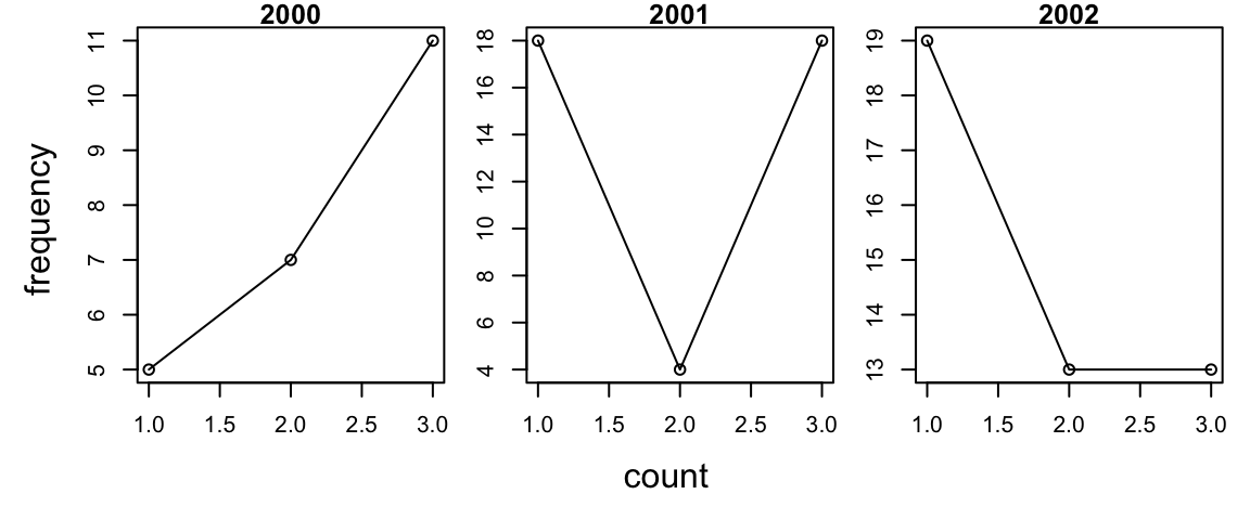
Nested chunking of the data
The basic syntax can be easily extended to break apart the data based on multiple columns:
baseball.dat <- subset(baseball, year > 2000) # data from the plyr package
x <- ddply(baseball.dat, c("year", "team"), summarize,
  homeruns = sum(hr))
head(x)
## year team homeruns
## 1 2001 ANA 4
## 2 2001 ARI 155
## 3 2001 ATL 63
## 4 2001 BAL 58
## 5 2001 BOS 77
## 6 2001 CHA 63Other useful options
Dealing with errors
You can use the failwith function to control how errors are dealt
with.
f <- function(x) if (x == 1) stop("Error!") else 1
safe.f <- failwith(NA, f, quiet = TRUE)
# llply(1:2, f)
llply(1:2, safe.f)
## [[1]]
## [1] NA
##
## [[2]]
## [1] 1Parallel processing
In conjunction with a package such as doParallel you can run your function
separately on each core of your computer. On a dual core machine this make
your code up to twice as fast. Simply register the cores and then set
.parallel = TRUE. Look at the elapsed time in these examples:
x <- c(1:10)
wait <- function(i) Sys.sleep(0.1)
system.time(llply(x, wait))
## user system elapsed
## 0.002 0.000 1.043system.time(sapply(x, wait))## user system elapsed
## 0.000 0.000 1.022library(doParallel)## Loading required package: foreach## Loading required package: iterators## Loading required package: parallelregisterDoParallel(cores = 2)
system.time(llply(x, wait, .parallel = TRUE))## user system elapsed
## 0.095 0.014 0.625So, why would I not want to use plyr?
plyr can be slow — particularly if you are working with very large
datasets that involve a lot of subsetting. Hadley is working on this and
an in-development version of plyr, dplyr, can run much faster (https://github.com/hadley/dplyr).
However, it’s important to remember that typically the speed that you
can write code and understand it later is the rate-limiting step.
A couple faster options:
Use a base R apply function:
system.time(ddply(baseball, "id", summarize, length(year)))## user system elapsed
## 0.271 0.002 0.276system.time(tapply(baseball$year, baseball$id,
function(x) length(x)))## user system elapsed
## 0.006 0.000 0.007Use the data.table package:
library(data.table)
dt <- data.table(baseball, key = "id")
system.time(dt[, length(year), by = list(id)])
## user system elapsed
## 0.077 0.001 0.010