A Gamma error distribution with a log link is a common family to fit GLMs with in ecology. It works well for positive-only data with positively-skewed errors. The Gamma distribution is flexible and can mimic, among other shapes, a log-normal shape. The log link can represent an underlying multiplicate process, which is common in ecology.
Here, I’ll fit a GLM with Gamma errors and a log link in four different ways. (1) With the built-in glm() function in R, (2) by optimizing our own likelihood function, (3) by the MCMC Gibbs sampler with JAGS, and (4) by the MCMC No U-Turn Sampler in Stan (the shiny new Bayesian toolbox toy).
I wrote this code for myself to make sure I understood what was going on during the fitting process, but I thought I’d share it here. When I’m learning a new method, I often find it useful to see the same problem solved using a method I know along with a method I’m learning.
There are multiple ways to parameterize the Gamma distribution in R. Here I’ve chosen to use the “rate” and “shape” parameters to match how it is parameterized in JAGS.
We’ll start by simulating some data:
set.seed(999)
N <- 100
x <- runif(N, -1, 1)
a <- 0.5
b <- 1.2
y_true <- exp(a + b * x)
shape <- 10
y <- rgamma(N, rate = shape / y_true, shape = shape)
Let’s look at what we just simulated:
plot(x, y)
lines(sort(x), y_true[order(x)])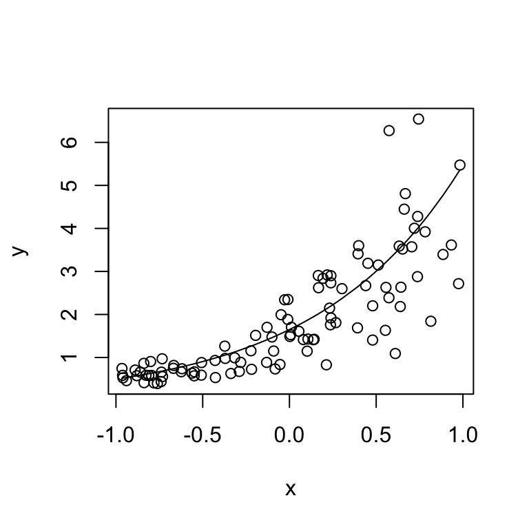
First, we’ll fit a model to our data with glm() to make sure we can recover the parameters underlying our simulated data:
m_glm <- glm(y ~ x, family = Gamma(link = "log"))
m_glm_ci <- confint(m_glm)
coef(m_glm)
## (Intercept) x
## 0.4355899 1.1652181That’s pretty close to our “true” simulated values. We’ll use these values as a reference for our methods below.
To make sure we understand what’s going on, we’ll write our own likelihood function and optimize the fit to the data ourselves with Ben Bolker’s mle2() function. You’ll need the bbmle library.
library("bbmle")## Loading required package: stats4nll_gamma <- function(a, b, logshape) {
linear_predictor <- a + b * x
# rate = shape / mean:
rate <- exp(logshape) / exp(linear_predictor)
# sum of negative log likelihoods:
-sum(dgamma(y, rate = rate, shape = exp(logshape),
log = TRUE))
}
(m_mle2 <- bbmle::mle2(nll_gamma,
start = list(a = rnorm(1), b = rnorm(1),
logshape = rlnorm(1))))##
## Call:
## bbmle::mle2(minuslogl = nll_gamma, start = list(a = rnorm(1),
## b = rnorm(1), logshape = rlnorm(1)))
##
## Coefficients:
## a b logshape
## 0.4356475 1.1651330 2.2458513
##
## Log-likelihood: -66.55One of the niceties built into mle2() is the ability to estimate profile likelihood intervals with a confint() function:
(m_mle2_ci <- confint(m_mle2))## 2.5 % 97.5 %
## a 0.3718561 0.5007131
## b 1.0506891 1.2794035
## logshape 1.9612353 2.5069835Now, we’ll use the same approach to fit our model, but this time via MCMC with JAGS:
library("R2jags")
m <- function() {
  # Priors:
  a ~ dnorm(0, 0.0001) # mean, precision = N(0, 10^4)
  b ~ dnorm(0, 0.0001)
  shape ~ dunif(0, 100)

  # Likelihood data model:
  for (i in 1:N) {
    linear_predictor[i] <- a + b * x[i]
    # dgamma(shape, rate) in JAGS:
    y[i] ~ dgamma(shape, shape / exp(linear_predictor[i]))
  }
}

m_jags <- R2jags::jags(data = list(N = N, y = y, x = x),
  parameters.to.save = c("a", "b", "shape"), model.file = m)
It’s important to inspect the output from any MCMC simulation to make sure the chains are mixing well and have converged. Rest assured that I have. Let’s extract the mean estimates:
m_jags_sims <- m_jags$BUGSoutput$sims.list
lapply(m_jags_sims, mean)[c(1, 2, 4)]
## $a
## [1] 0.436478
##
## $b
## [1] 1.163562
##
## $shape
## [1] 9.446129And plot, as an example, the density of MCMC samples for the parameter b:
plot(density(m_jags_sims$b), main = "")
We’ll also calculate 95% credible intervals. We’ll use HPD intervals (highest probability density):
(m_jags_ci <- coda::HPDinterval(coda::as.mcmc(m_jags_sims$b)))## lower upper
## var1 1.045871 1.277708
## attr(,"Probability")
## [1] 0.95Now with Stan:
library(rstan)
stan_code <- "
data {
  int<lower=0> N;
  vector[N] x;
  vector[N] y;
}
parameters {
  real a;
  real b;
  real<lower=0.001,upper=100> shape;
}
model {
  a ~ normal(0,100);
  b ~ normal(0,100);
  for(i in 1:N)
    y[i] ~ gamma(shape, (shape / exp(a + b * x[i])));
}
"
m_stan <- stan(model_code = stan_code,
    data = list(x = x, y = y, N = N))
We’ll look at the means of each estimated parameter:
lapply(extract(m_stan), mean)[c(1, 2, 3)]## $a
## [1] 0.4368692
##
## $b
## [1] 1.16558
##
## $shape
## [1] 9.470829And we’ll extract the 95% HPD interval again:
stan_b <- extract(m_stan)$b
(m_stan_ci <- coda::HPDinterval(coda::as.mcmc(as.vector(stan_b))))
## lower upper
## var1 1.04786 1.280054
## attr(,"Probability")
## [1] 0.95Finally, we’ll plot the four fits to show that they are all qualitatively the same:
par(mfrow = c(1, 2), las = 1, mgp = c(2, 0.5, 0),
  tcl = -0.15, mar = c(4, 3, 0, 0.5), oma = c(0, 0, 1, 1))

# left panel:
plot(x, y)
lines(x[order(x)], y_true[order(x)], col = "#00000050",
  lty = 2, lwd = 2)
X <- seq(min(x), max(x), length.out = 100)
lines(X, exp(coef(m_glm)[1] + coef(m_glm)[2] * X),
  col = "red")
lines(X, exp(coef(m_mle2)[1] + coef(m_mle2)[2] * X),
  col = "blue")
lines(X, exp(mean(m_jags_sims$a) + mean(m_jags_sims$b) * X),
  col = "green")
lines(X, exp(get_posterior_mean(m_stan)[1,5] +
    get_posterior_mean(m_stan)[2,5] * X), col = "black")

# right panel:
plot(1, 1, xlim = c(1, 4), ylim = c(0.5, 2), type = "n",
  xaxt = "n", xlab = "", ylab = "Estimate of b")
abline(h = b, col = "#00000050", lwd = 2, lty = 2)
points(1, coef(m_glm)[2])
segments(1, m_glm_ci[2, 1], 1, m_glm_ci[2, 2])
points(2, coef(m_mle2)[2])
segments(2, m_mle2_ci[2, 1], 2, m_mle2_ci[2, 2])
points(3, mean(m_jags_sims$b))
segments(3, m_jags_ci[1, 1], 3, m_jags_ci[1, 2])
points(4, get_posterior_mean(m_stan)["b", "mean-all chains"])
segments(4, m_stan_ci[1, 1], 4, m_stan_ci[1, 2])

axis(1, at = c(1, 2, 3, 4), labels = c("glm()", "mle2()",
    "JAGS", "Stan"))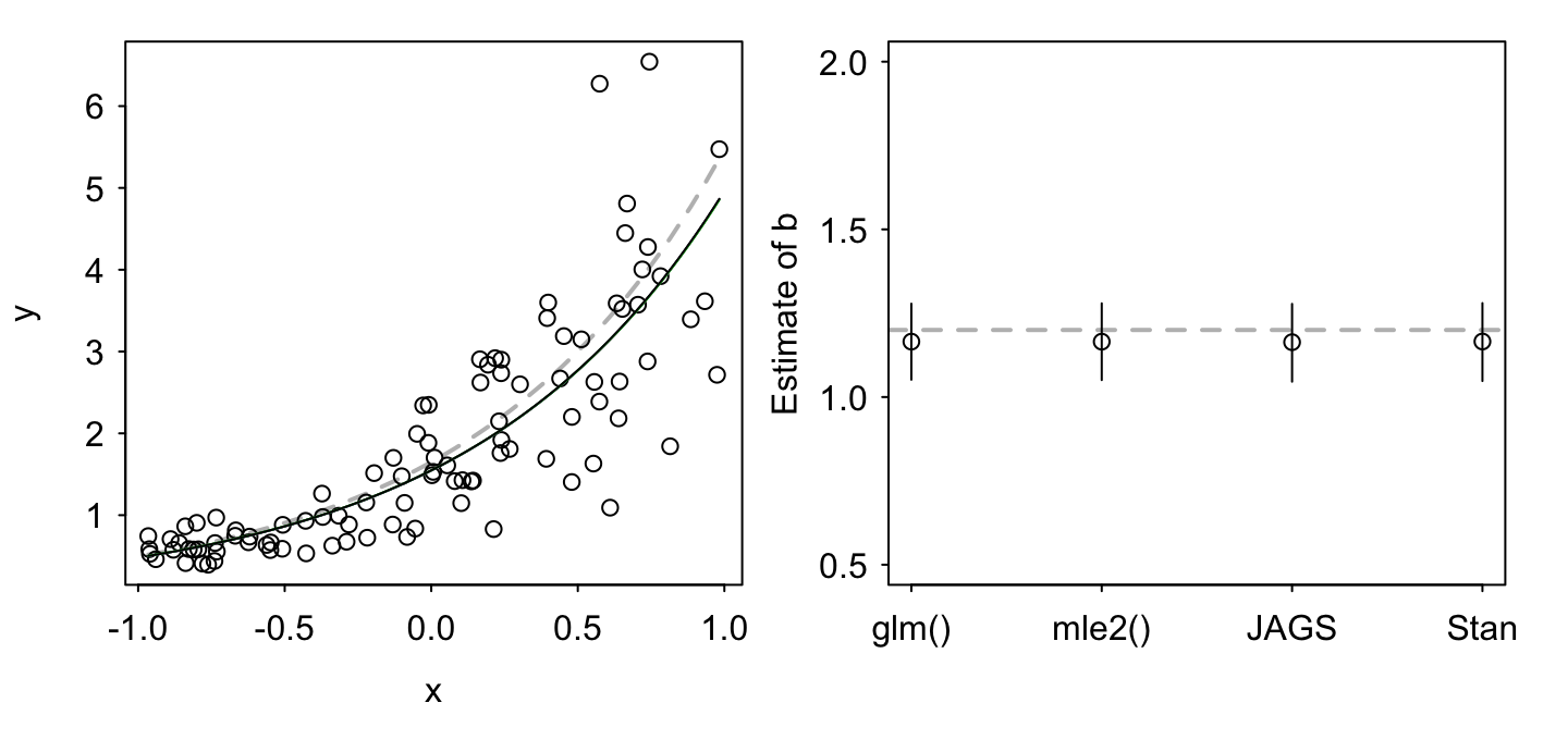
Take home messages
As expected, all four methods give us a similar result (although some with different interpretations — Bayesian vs. frequentist).
Simulation, as always, is a great way to understand statistical models.
Although we call it a “log link”, if we’re working with the Gamma distribution directly, we exponentiate the linear predictor instead of logging the data. This ensures that we don’t propose negative mean values to the Gamma distribution.
There are multiple ways to parameterize the Gamma distribution, so it’s important to pay attention when moving between languages and functions.
As with many optimization exercises, we can force a term (here shape) to be positive by fitting in log-space. Hence, using logshape and exponentiating within the optimization function for some of the examples. This creates a smooth likelihood or probability surface near the boundaries that optimization algorithms can better navigate.