Zero inflation
Ecologists often run into a scenario where their response data have more zeros than expected if the process generating their data was purely from a standard probability distribution. For example, there might be more zeros than you’d expect from a negative binomial distribution with a given mean. Two common methods for dealing with zero-inflated data are:
Modelling a zero-inflation parameter that represents the probability a given zero comes from the main distribution (say the negative binomial distribution) or is an excess zero.
Modelling the zero and non-zero data with one model and then modelling the non-zero data with another. This is often called a “hurdle model”.
So, zero-inflation models separate the zeros into “true” and “extra” categories.
Hurdle models model the zeros and non-zeros as two separate processes.
Zero-inflation models may be more elegant and informative if the same predictors are thought to contribute to the extra and real zeros.
Hurdle models can be useful in that they allow you to model the zeros and non-zeros with different predictors or different roles of the same predictors. Maybe one process leads to the zero/non-zero data and another leads to the non-zero magnitude.
For count data (probably the most typical situation where zero inflation is a problem), there are already a variety of R packages to fit either zero-inflated or hurdle models. E.g. pscl for models without random effects, glmmADMB for models with or without random effects, and MCMCglmm for Bayesian models with or without random effects.
Zero-inflated continuous data
Sometimes ecologists end up with a response dataset that is positive and continuous but has zero inflation. (Technically, any number of zeros is “zero inflation” for probability distributions that only represent non-zero positive values.) There are probably many scenarios that can result in this kind of data. Sometimes the “zeros” may not really be zeros but just really small values that weren’t measured. But there are also plausible scenarios where the zeros are real. For example, if the response variable is biomass at a given site, it’s possible there were just no individuals at some sites. If you want to model the biomass with a distribution such as the log-normal or Gamma, these distributions don’t allow for zero values. One solution is to model the zeros separately from the non-zeros in a binomial-Gamma hurdle model.
This post illustrates a small simulated example of one of these hurdle models where we estimate an intercept only. I describe how to fit the model, interpret the coefficients, and generate predictions with confidence intervals.
Note that the methods as illustrated here don’t apply exactly to count-based hurdle models since count-based models require a truncated count distribution. I.e., they need to account for the fact that the negative binomial or Poisson distribution can represent zeros too, but these zeros were already accounted for in the binomial model. Since the Gamma distribution can not represent zero values we don’t need to worry about that. Count hurdle models can be fitted with the packages mentioned above.
Fitting the models
We’ll start by simulating some data and plotting it. First we’ll simulate a binomial process (0 or 1) with a probability of a non-zero value (1) of 0.7. Then we’ll simulate a Gamma process with a shape (mean) of 0.4.
set.seed(1)
x <- 1:150
y <- rbinom(length(x), size = 1, prob = 0.7)
y <- y * rgamma(length(x), shape = 0.4)
non_zero <- ifelse(y > 0, 1, 0)
d <- data.frame(x, y, non_zero)
head(d)
## x y non_zero
## 1 1 0.08735883 1
## 2 2 0.28772983 1
## 3 3 0.05730738 1
## 4 4 0.00000000 0
## 5 5 1.07186263 1
## 6 6 0.00000000 0library(ggplot2)
p <- ggplot(d, aes(x, y, colour = as.factor(non_zero))) + geom_point()
print(p)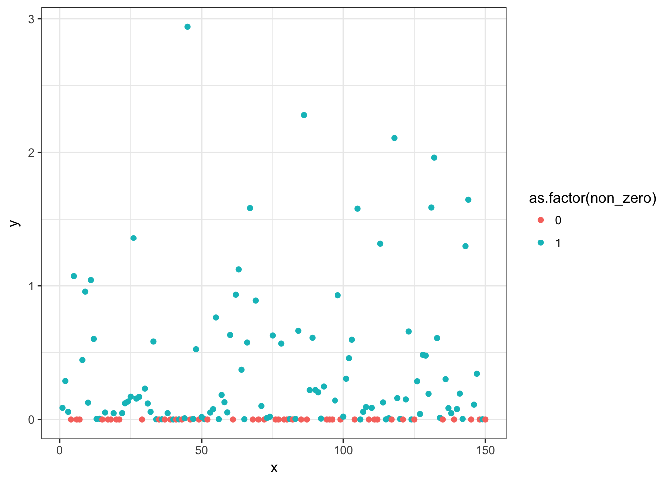
Now we’ll fit a logistic regression to predict the probability of a non-zero value and a Gamma GLM with a log link to predict the mean of the non-zero data.
m1 <- glm(non_zero ~ 1, data = d, family = binomial(link = logit))
m2 <- glm(y ~ 1, data = subset(d, non_zero == 1), family = Gamma(link = log))
We’ll extract the coefficients and show the 95% confidence intervals (derived from profile likelihoods). Note that the Gamma coefficients come out on a log-scale and we’ll exponentiate them as we go. The logistic regression coefficients come out on the logit scale and we’ll inverse that link as we go as well.
(bin_coef <- plogis(coef(m1)[[1]])) # close to prob = 0.7 as specified## [1] 0.7066667(gamma_coef <- exp(coef(m2)[[1]])) # close to shape = 0.4 as specified## [1] 0.4075046(plogis(confint(m1)))## 2.5 % 97.5 %
## 0.6307292 0.7756071(exp(confint(m2)))## 2.5 % 97.5 %
## 0.3158070 0.5384332So, we’ve managed to recover our simulated means. The logistic model indicates that the mean probability of observing a non-zero value is about 0.7. The Gamma model indicates that given we have observed a non-zero value, the mean of our response value y is about 0.4.
Predictions
We could plot these coefficients along with their confidence intervals. We could also plot predictions for these two separate processes. For example, we’ll plot the predictions along with confidence intervals for these two models here. Note that because we only modelled an intercept, we’ll get the same predictions regardless of the data to be predicted on.
pred1 <- predict(m1, se = TRUE, type = "link")
pred2 <- predict(m2, se = TRUE, type = "link")

# Zero/non-zero binomial model:
ggplot(d, aes(x, non_zero)) + geom_point() +
  geom_hline(yintercept = plogis(pred1$fit)) +
  geom_hline(yintercept = plogis(pred1$fit +
      c(1.96, -1.96) * pred1$se.fit),
    colour = "darkgrey")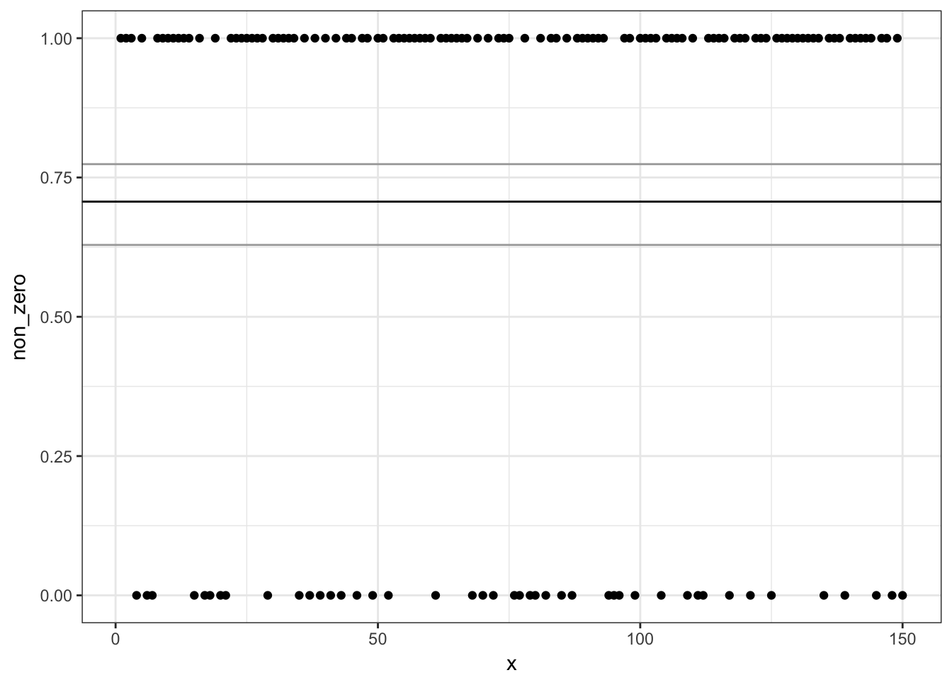
# Non-zero Gamma model:
ggplot(subset(d, non_zero == 1),
  aes(x, y)) + geom_point() +
  geom_hline(yintercept = exp(pred2$fit)) +
  geom_hline(yintercept = exp(pred2$fit +
      c(1.96, -1.96) * pred2$se.fit),
    colour = "darkgrey")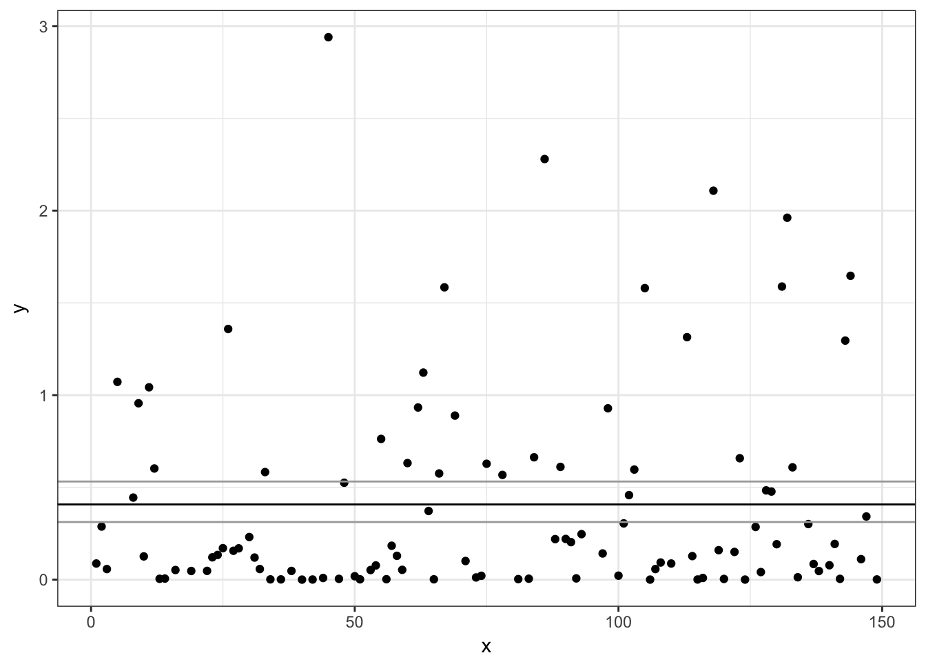
We can also check the predictions incorporating both the binomial and Gamma models. To do that, we take the two means, add them on a log scale and re-exponentiate them. We can check that the predicted mean (intercept) matches the arithmetic mean.
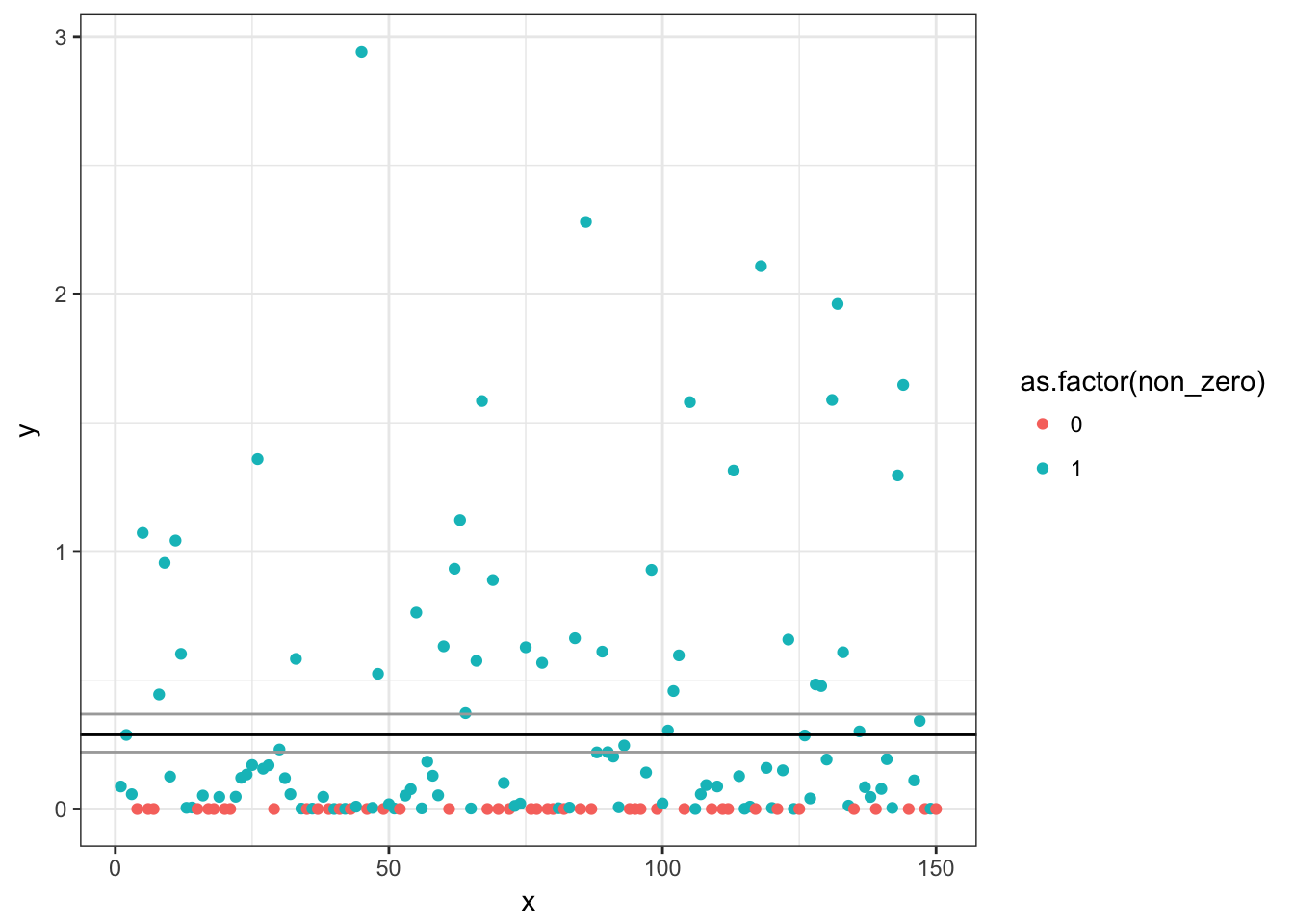
(pred <- exp(log(bin_coef) + log(gamma_coef)))## [1] 0.2879699mean(d$y) # same## [1] 0.2879699p + geom_hline(yintercept = pred)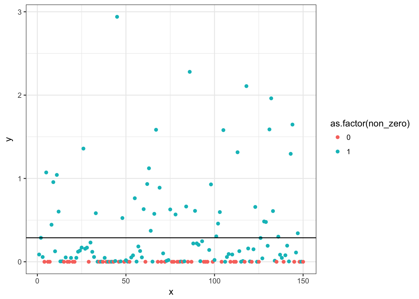
Prediction confidence intervals
Let’s derive confidence intervals on our predictions. One way to do that is using a non-parametric bootstrap method. To do that we’ll define a little function that carries out our hurdle model as above. boot requires that the function’s first argument be the data and the second argument be a vector of row indices for each bootstrap replicate. The function should return the statistic we want to bootstrap (here the prediction).
We’ll run 500 replicates. In a real analysis you’d want to make sure you’d run enough replicates that the estimates had stabilized. You could test this by increasing the number of replicates until you start getting the same confidence intervals (to whatever level of precision you are interested in) regardless of whether you add more replicates.
We’ll use the bias-corrected confidence intervals. Read the documentation for boot.ci and the recommended references in the documentation for details.
hurdle_fn <- function(data, i) {
  dat_boot <- data[i, ]
  m1 <- glm(non_zero ~ 1, data = dat_boot,
    family = binomial(link = logit))
  m2 <- glm(y ~ 1, data = subset(dat_boot, non_zero == 1),
    family = Gamma(link = log))
  bin_coef <- plogis(coef(m1)[[1]])
  gamma_coef <- exp(coef(m2)[[1]])
  exp(log(bin_coef) + log(gamma_coef))
}

library(boot)
b <- boot(d, hurdle_fn, R = 500)
b.ci <- boot.ci(b, type = "bca")
print(b.ci)
## BOOTSTRAP CONFIDENCE INTERVAL CALCULATIONS
## Based on 500 bootstrap replicates
##
## CALL :
## boot.ci(boot.out = b, type = "bca")
##
## Intervals :
## Level BCa
## 95% ( 0.2207, 0.3683 )
## Calculations and Intervals on Original Scale
## Some BCa intervals may be unstablep + geom_hline(yintercept = pred) +
geom_hline(yintercept = b.ci$bca[c(4:5)],
colour = "darkgrey")