I’ve encountered a number of people wondering about centering and scaling predictors in the context of model averaging. Here, centering refers to subtracting the mean and scaling refers to dividing by some measure of variability (usually one or two standard deviations).
First of all, if you haven’t already, go read the paper Simple means to improve the interpretability of regression coefficients by Holger Schielzeth. This paper is a wealth of useful information.
Bottom line, if you are going to average coefficients across models with and without interactions you’re going to get gibberish unless you center your predictors by subtracting the mean. This is true across continuous, binary, and multi-level factor predictors, although setting up centered factor predictors can take an extra step.
Whether or not averaging coefficient values across models is a good idea is a separate topic that I won’t get into here. Just realize that subscribing to the church of coefficient averaging is not the only way and there are also good arguments for three alternatives: maintaining multiple models, model selection (e.g. as often suggested in Zuur’s books), or, assuming reasonable power, fitting the most complicated model you can justify and interpret and drawing inference from that model (e.g. Andrew Gelman). After all, removing a predictor is equivalent to assuming the coefficient for that predictor is precisely zero, which is a strong assumption in itself. (This last philosophy often works best in Bayesian context where weakly informative priors are a possibility.)
First, we’ll simulate some data. b0 is an intercept, b1 a slope on a continuous predictor, b2 a binary factor coefficient, and b1.2 an interaction coefficient between b1 and b2.
set.seed(999)
b0 <- 1.4 # intercept
b1 <- 0.2 # continuous slope
b2 <- 1.7 # factor level 1 coefficient
b1.2 <- 0.5 # interaction between b1 and b2
sigma <- 2.0 # residual standard deviation
N <- 25 # number of data points

x1 <- runif(N, 0, 20) # continuous predictor data
x2 <- rbinom(N, size = 1, prob = 0.4) # binary predictor data

# generate response data:
y <- rnorm(N, mean = b0 +
  b1 * x1 +
  b2 * x2 +
  x1 * x2 * b1.2,
  sd = sigma)
dat <- data.frame(x1, x2, y)
head(dat)
## x1 x2 y
## 1 7.781428 1 9.831531
## 2 11.661214 0 1.518768
## 3 1.893314 1 2.655639
## 4 17.052625 1 11.928647
## 5 15.734935 0 4.293629
## 6 2.386845 0 6.642697Let’s look at the data we created:
library(ggplot2)
ggplot(dat, aes(x1, y, colour = as.factor(x2))) + geom_point()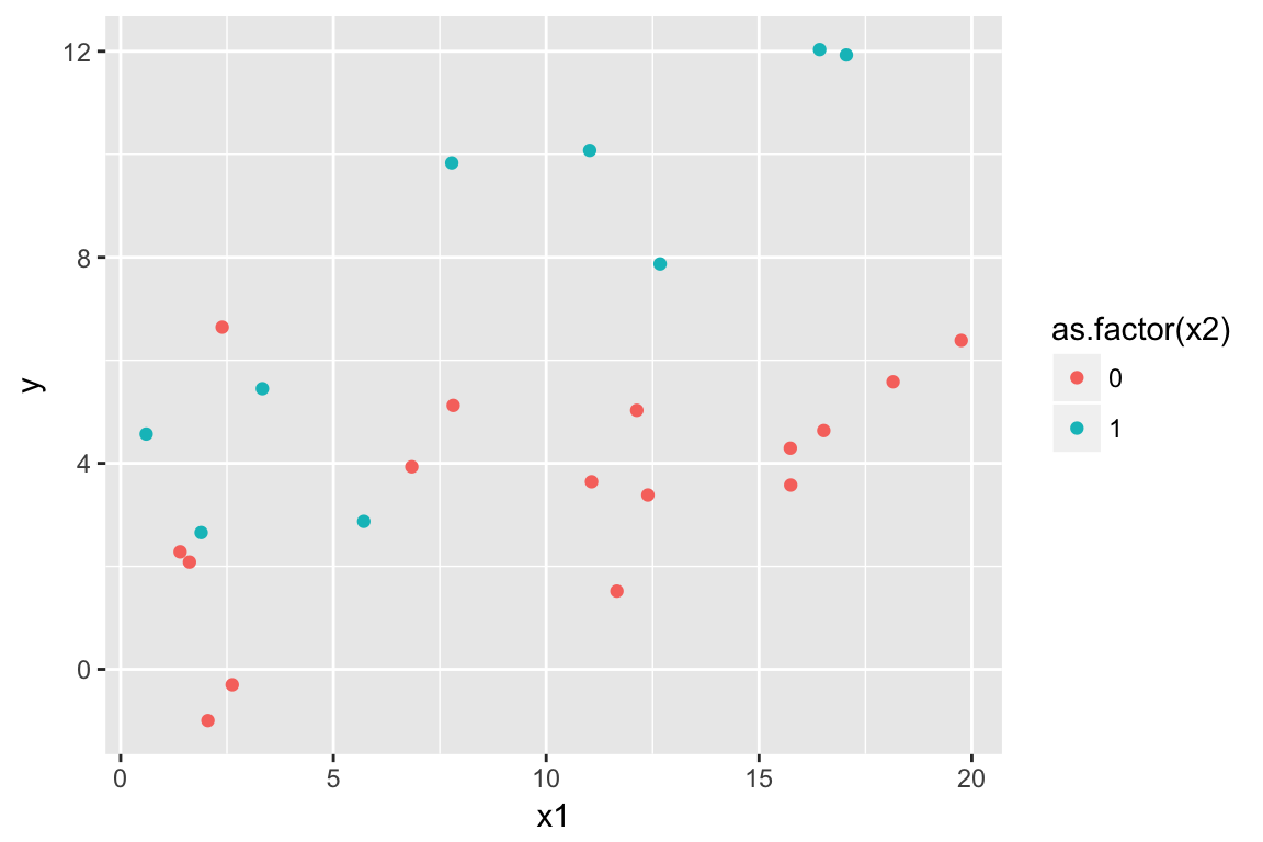
Now, we’ll fit a model with and without an interaction and look at the coefficients:
m <- lm(y ~ x1 * x2, data = dat)
m_no_inter <- lm(y ~ x1 + x2, data = dat)
round(coef(m), 2)
## (Intercept) x1 x2 x1:x2
## 1.72 0.19 1.27 0.34round(coef(m_no_inter), 2)## (Intercept) x1 x2
## 0.61 0.30 4.33Notice how the main effects (everything except the interaction) change dramatically when the interaction is removed. This is because when the interaction is included the main effects are relevant to when the other predictors are equal to 0. I.e. x1 = 0 or the binary predictor x2 is at its reference 0 level. But, when the interaction is excluded the main effects are relevant when the other predictors are at their mean values. So, if we center, the main effects will represent the same thing in both cases:
dat$x2_cent <- dat$x2 - mean(dat$x2)
dat$x1_cent <- dat$x1 - mean(dat$x1)
m_center <- lm(y ~ x1_cent * x2_cent, data = dat)
m_center_no_inter <- lm(y ~ x1_cent + x2_cent,
  data = dat)
round(coef(m_center), 2)
## (Intercept) x1_cent x2_cent x1_cent:x2_cent
## 5.07 0.31 4.48 0.34round(coef(m_center_no_inter), 2)## (Intercept) x1_cent x2_cent
## 4.96 0.30 4.33Notice that the intercept, x1, and x2 coefficient estimates are now similar regardless of whether the interaction is included. Now, because we’ve centered the predictors, the predictors equal zero at their mean. So, the main effects are estimating approximately the same thing regardless of whether we include the interaction. In other words, adding the interaction adds more predictive information but doesn’t modify the meaning of the main effects.
Here’s an illustration:
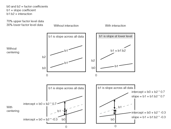
Illustration of centering interactions
A 3-level factor example
Now, let’s repeat the above with a three-level factor predictor to make sure it’s clear how it works.
set.seed(999)
b0 <- 1.4 # intercept
b1 <- 0.2 # continuous slope
b2 <- 1.7 # factor level 0-1 coefficient
b3 <- 2.9 # factor level 0-2 coefficient
b1.2 <- 0.5 # interaction between b1 and b2
b1.3 <- 0.9 # interaction between b1 and b3
sigma <- 2.0 # residual standard deviation
N <- 30 # number of data points

x1 <- runif(N, 0, 20) # continuous predictor data
# 3-factor predictor data:
f <- sample(c(1, 2, 3), N, replace = TRUE)

x2 <- ifelse(f == 2, 1, 0)
x3 <- ifelse(f == 3, 1, 0)

y <- rnorm(N, mean = b0 +
  b1 * x1 +
  b2 * x2 +
  b3 * x3 +
  x1 * x2 * b1.2 +
  x1 * x3 * b1.3,
  sd = sigma)

dat <- data.frame(x1, x2, x3, y,
  f = as.factor(f))
head(dat)
## x1 x2 x3 y f
## 1 7.781428 0 0 7.721614 1
## 2 11.661214 0 0 4.934795 1
## 3 1.893314 1 0 4.784042 2
## 4 17.052625 1 0 17.197900 2
## 5 15.734935 1 0 13.620830 2
## 6 2.386845 0 1 2.698056 3ggplot(dat, aes(x1, y, colour = f)) + geom_point()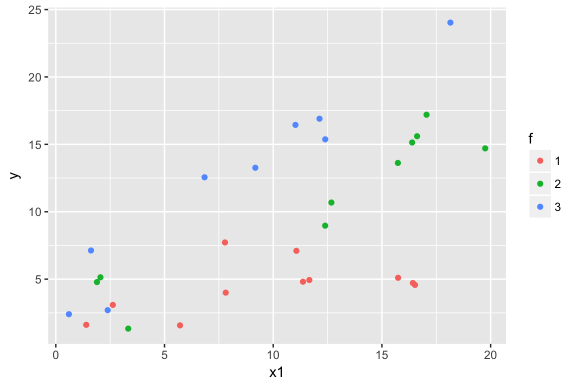
Now we’ll fit the model. First with factor() notation:
m2 <- lm(y ~ x1 * f, data = dat)
t(round(coef(m2), 2))
## (Intercept) x1 f2 f3 x1:f2 x1:f3
## [1,] 2.68 0.18 -0.81 -0.04 0.57 0.99And now with “dummy” variable notation. This will make centering in the next step easier:
m2.1 <- lm(y ~ x1 * x2 + x1 * x3, data = dat)
t(round(coef(m2.1), 2))
## (Intercept) x1 x2 x3 x1:x2 x1:x3
## [1,] 2.68 0.18 -0.81 -0.04 0.57 0.99Notice we get the same estimates.
Now, let’s compare to a model without the interaction before we center the data:
m2.1_no_inter <- lm(y ~ x1 + x2 + x1 + x3, data = dat)
t(round(coef(m2.1_no_inter), 2))
## (Intercept) x1 x2 x3
## [1,] -2.48 0.71 4.85 8.95The main effects look dramatically different. Again, if we model averaged here across models with and without the interaction, we’d be getting gibberish.
Now, we’ll fit the same model with centered predictors:
dat$x1_cent <- dat$x1 - mean(dat$x1)
dat$x2_cent <- dat$x2 - mean(dat$x2)
dat$x3_cent <- dat$x3 - mean(dat$x3)
m2.2 <- lm(y ~ x1_cent * x2_cent + x1_cent * x3_cent,
  data = dat)
m2.2_no_inter <- lm(y ~ x1_cent + x2_cent + x3_cent,
  data = dat)
Again, notice that the main effects stay fairly consistent regardless of whether we include the interaction because they are estimated across the centered three-level factor:
t(round(coef(m2.2), 2)) # no interaction ## (Intercept) x1_cent x2_cent x3_cent x1_cent:x2_cent x1_cent:x3_cent
## [1,] 9.09 0.67 4.87 9.86 0.57 0.99t(round(coef(m2.2_no_inter), 2)) # with interaction## (Intercept) x1_cent x2_cent x3_cent
## [1,] 8.91 0.71 4.85 8.95You can see how this works across multiple model comparisons using the MuMIn::dredge() function on any one of the above models.
So, if you’re going to average across models with and without interactions, centering the predictors is important. Even if you’re not going to be averaging or comparing coefficient values across models with and without interactions, centering predictors can be useful for computational and interpretation reasons, but that’s a separate topic.
Plotting the predictions
Say we wanted to plot the predicted response from our model on new data. This isn’t quite as simple as normal once we’ve centered our predictors and coded the factor levels as centered dummy variable comparisons.
We’ll make predictions at each of the 3 levels. Note how we create these levels through the 3 valid combinations of high and low values of our dummy variables. We can’t just use expand.grid() and get all combinations of our dummy variables.
x1_cent <- seq(-10, 10, length.out = 100)
newdata1 <- data.frame(x1_cent = x1_cent,
x2_cent = min(dat$x2_cent), x3_cent = min(dat$x3_cent))
newdata2 <- data.frame(x1_cent = x1_cent,
x2_cent = max(dat$x2_cent), x3_cent = min(dat$x3_cent))
newdata3 <- data.frame(x1_cent = x1_cent,
x2_cent = min(dat$x2_cent), x3_cent = max(dat$x3_cent))
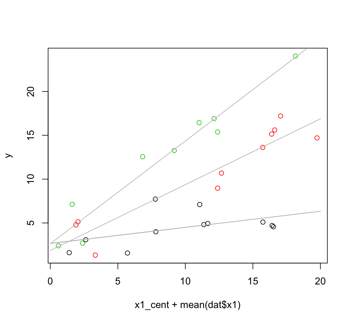
newdata <- rbind(newdata1, newdata2, newdata3)Now we make our predictions and plot the predictions. We’ll undo the centering of the x1 variable here by adding the mean of the original data:
newdata$pred <- predict(m2.2, newdata = newdata)
with(dat, plot(x1_cent + mean(dat$x1), y, col = f))
plyr::d_ply(newdata, "x2_cent", function(x) {
  with(x, lines(x1_cent + mean(dat$x1), pred, col = "grey"))
  })
Calculating slopes and standard errors at interaction levels
Currently, our factor variable f has three levels. Our estimate b1 represents the slope across the mean of the factors. However, we might want to present the slope with confidence intervals at each level of factor f.
Calculating the slope coefficients is fairly easy but the standard errors require a bit more math. The trick is to correctly combine the coefficient variances (or equivalently the squared standard errors) with the covariances between coefficients.
The way we combine the standard errors is the same way we combine the standard deviation of any normal distributions. For the case:
N1 ~ N(mu1, sigma1)
N2 ~ N(mu2, sigma2)
where mu represents the mean, sigma represents the standard deviation, and N represents a normal distribution.
We can calculate the combination of these two distributions multiplied by the constants a and b as: (we’ll this new distribution N3)
N3 = a * N1 + b * N2
N3 ~ N(mu3, sigma3)
mu3 = a * mu1 + b * mu2
sigma3 = sqrt(a^2 * sigma1^2 + b^2 * sigma2^2 +
  2 * ab * cov(ab))
First, to illustrate combining the coefficient means, here’s an example plotting the predictions by specifying the intercept and slopes. The first line in each of these abline function calls represents the intercepts and each factor level and the second line represents the slopes. As before, notice how we get these slopes by turning the two indicator columns to low or high values.
with(dat, plot(x1_cent, y, col = f))
b <- coef(m2.2)
se <- summary(m2.2)$coef[,2]
# The intercept and slope for the first level of the factor f:
abline(a = b[1] + b[3]*-0.333 + b[4] * -0.3,
  b = b[2] + b[5]*-0.333 + b[6] * -0.3, col = 1)
# And the second level:
abline(a = b[1] + b[3]*0.667 + b[4] * -0.3,
  b = b[2] + b[5]*0.667 + b[6] * -0.3, col = 2)
# And the third:
abline(a = b[1] + b[3]*-0.333 + b[4] * 0.7,
  b = b[2] + b[5]*-0.333 + b[6] * 0.7, col = 3)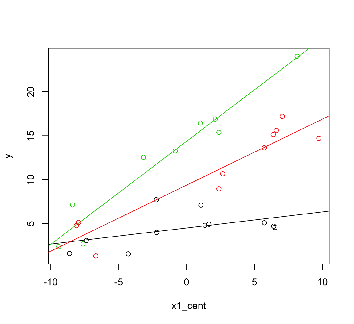
Before we calculate the standard errors on the slope at the three factor levels let’s return to a more straightforward parameterization so we know what we’re aiming for. I’ll re-write the model here for clarity:
m2 <- lm(y ~ x1 * f, data = dat)
b <- coef(m2)
se <- summary(m2)$coef[,2]

# Slopes:
with(dat, plot(x1, y, col = f))
abline(a = b[1], b = b[2], col = 1)
abline(a = b[1] + b[3], b = b[2] + b[5], col = 2)
abline(a = b[1] + b[4], b = b[2] + b[6], col = 3)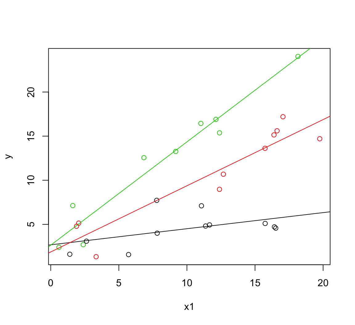
# SEs on those slopes:
# (as in Schielzeth 2010 Methods Ecol. Evol.)
se[2]
## x1
## 0.1114734sqrt(se[5]^2 - se[2]^2)## x1:f2
## 0.09118352sqrt(se[6]^2 - se[2]^2)## x1:f3
## 0.1117044Now, let’s derive those same standard errors for the centered version. We’ll start be extracting the standard errors and covariances of the coefficients. Then we’ll combine them. Although we could do this more elegantly, we’ll write it out in full to make it obvious what’s happening.
se <- summary(m2.2)$coef[,2]
x1x2_low <- min(dat$x2_cent)
x1x2_high <- max(dat$x2_cent)
x1x3_low <- min(dat$x3_cent)
x1x3_high <- max(dat$x3_cent)
vcov_x1_x1x2 <- vcov(m2.2)[5, 2]
vcov_x1_x1x3 <- vcov(m2.2)[6, 2]
vcov_x1x2_x1x3 <- vcov(m2.2)[6, 5]
se_x1 <- se[2]
se_x1x2 <- se[5]
se_x1x3 <- se[6]
Standard error on the slope at the first factor level:
as.numeric(
sqrt(x1x2_low^2 * se_x1x2^2 +
     x1x3_low^2 * se_x1x3^2 +
     se_x1^2 +
     2 * x1x2_low * vcov_x1_x1x2 +
     2 * x1x3_low * vcov_x1_x1x3 +
     2 * x1x2_low * x1x3_low * vcov_x1x2_x1x3)
)
## [1] 0.1114734This matches the version from the uncentered model:
summary(m2)$coef[2,2] ## [1] 0.1114734And the second level:
as.numeric(
sqrt(x1x2_high^2 * se_x1x2^2 +
     x1x3_low^2 * se_x1x3^2 +
     se_x1^2 +
     2 * x1x2_high * vcov_x1_x1x2 +
     2 * x1x3_low * vcov_x1_x1x3 +
     2 * x1x2_high * x1x3_low * vcov_x1x2_x1x3)
)
## [1] 0.09118352And the third level:
as.numeric(
sqrt(x1x2_low^2 * se_x1x2^2 +
     x1x3_high^2 * se_x1x3^2 +
     se_x1^2 +
     2 * x1x2_low * vcov_x1_x1x2 +
     2 * x1x3_high * vcov_x1_x1x3 +
     2 * x1x2_low * x1x3_high * vcov_x1x2_x1x3)
)
## [1] 0.1117044Again, comparing to the uncentered version, they match:
se <- summary(m2)$coef[,2]
sqrt(se[5]^2 - se[2]^2)
## x1:f2
## 0.09118352sqrt(se[6]^2 - se[2]^2)## x1:f3
## 0.1117044Whether or not you center your predictors, transforming your factor coefficient interactions like the above can be a powerful way of displaying data. For example see Figure 1 in O’Regan et al. 2014, Ecology, 95(4) where we use this method to illustrate the effect of climate warming and drying on four responses across three amphibian species. Each panel represents a single model and we’ve adjusted the coefficients so that each effect is with respect to zero instead of with respect to another factor level. If this kind of presentation of the results is all you’re after, then there’s no need to center the factor levels. If, however, you also want to apply model averaging to coefficient values that include interactions, you will need to center your predictors and combine the coefficients as in the above example.